Population Dynamics Model

Deer, Vegetation, Predators

SC "96

Prepared by Jackie Snow

The purpose of this tutorial is to provide the beginning Stella modeler with the expertise to develop a simple model of population dynamics using Stella II. The basis for this document is found in "Getting Started with Stella II: A Hands-On Experience" from the Stella software.

Studies of diverse populations have shown that there are a few common patterns of growth which emerge repeatedly. "Overshoot and Collapse" is one such pattern. We will construct a model of a deer population to see if we can discover what relationships are responsible for generating this pattern.

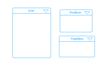
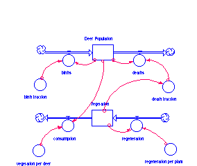
Open Stella II and select New from the file menu. Using the process frame building block (left on the palette), create the High-level Map seen below. The 3 players in our model are deer, predators, and vegetation.

Label each frame.

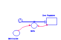
Click on the downward-pointing area in the header of the Deer process frame. This is what a sector looks like on the Diagram Layer. Inside this frame, we will put all of the parts of the model relating to deer. Begin creating the map shown below using the building blocks at the left of the palette. You will use 1 stock, 1 flow, 1 converter, and 2 connectors. Make sure your flow is connected to the stock; there should only be one cloud.

Modeling: Round 1

We are now ready to bring this map to life via simulation and animation. The Stella II software already has begun this process by automatically creating the equation framework needed to do the basic "accounting" for the system. Click on the downward-pointing arrowhead located above the globe icon on the left border. For each accumulation, represented by a stock, and the associated set of flows, the software generated a generic equation. The equation says, in words: "What you have now, is what you had an instant ago {i.e., 1 dt in the past), + whatever flowed in over the instant, - whatever flowed out over the instant." The software automatically assigns + and - signs based on the direction of the flow arrowheads in relation to the stock.

In order to simulate, the software needs to know "How much is in each accumulation at the outset of the simulation?" It also needs to know "What is the flow volume for each of the flows?" Both will be answered as we move from the mapping to the modeling phase. Click once on the upward-pointing arrowhead on the left frame of the equations window. This returns you to the diagram. Click once on the Globe icon to shift to the modeling mode (the icon changes to X² and a ? will appear in each icon on the diagram). The ?'s indicate the need for information to enable simulation of the model.

Births depend on Deer Population since an increase in deer will cause an increase in deer births. To show this dependence use a connector to link Deer Population to births. Double-click on births flow regulator . Click in the equation (Deer Population *birth fraction) by clicking on the respective variables in the Required Inputs List. Click OK to exit. Note the ? no longer appears on the births flow regulator.

To determine an initial value for our Deer Population at the beginning of the simulation, double click on Deer Population and click in or type 100. Click OK. To define the birth fraction, assume 2 births for every 10 deer in the population = a birth fraction of .2. Double click on the birth fraction converter and click in or type .2. Click OK to exit the birth fraction dialog.

Simulating: Round 1

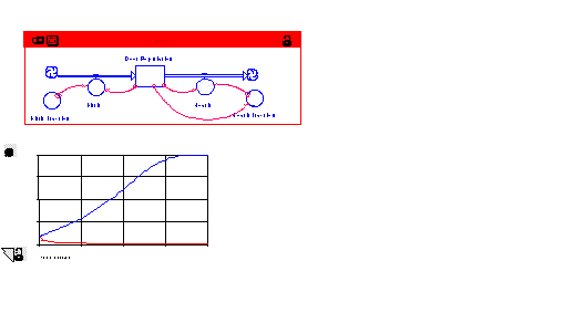
Click on the Run icon to open the run controller. Create a graph by selecting the graph pad icon from the objects palette. Click once on the diagram, to deposit a graph pad in that spot. Pin it in place using the push pin in the upper left corner. Double-click on the blank graph pad page. Move Deer Population from the available list to the selected list within the dialog. Click OK

Choose Time Specs... from the Run menu. Click the radio button next to Years in the list under the heading "Unit of time:" Years will become the time unit on the graph. Click OK.

Run the model and watch the graph of Deer Population unfold over time. The scale for Deer Population should run from 100 to 1040.13. To specify a more precise scale for the graph double-click on the graph. Click once on Deer Population in the selected list. While Deer Population is selected, click once on the two-headed arrow to the right of Deer Population. Horizontal lines appear above and below the arrow. This indicates that you can select a local scale for the variable. Type "0" in the Min box and "1500" in the Max box. Click Set. Click OK. You have a new scale for your graph.

To see actual numbers create a Table. Select the Table Pad icon from the Objects palette. Place it by the Graph Pad icon. Double-click the resulting page and enter the births flow and Deer Population stock into the Selected list. Click OK, and Run the model. The Table results will show you how Stella II is calculating the values for the entities you selected.

Modeling: Round 2

Recall the "overshoot and collapse" dynamic we are seeking to represent? The graph and table indicate something is missing from our model. Deer Population is growing exponentially with nothing to check it's progress. There is no collapse to the pattern. In order to generate a collapse, there must be a check on Deer Population growth. Add a deaths flow and a death fraction to the diagram. See the diagram below.

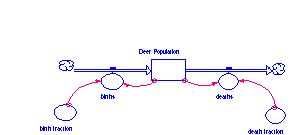
Define these two new entities. Open the deaths flow and click in Deer Population from the Required Inputs list. Then click * and click in death fraction. Click OK. Set the death fraction to .02.

Simulating: Round 2

How do you think the addition of a deaths outflow will alter the pattern traced by Deer Population? Run the model and observe the new behavior on the graph. Deer Population continues to grow exponentially. We have slowed growth but have not produced collapse.

To examine the sensitivity of model performance to a variation in model parameter values Stella II has a feature called "Sensitivity Analysis". If the value of the death fraction is too small we can test various values for death fraction to see how they affect the pattern traced by Deer Population. Select Sensi Specs. from the Run Menu. Enter death fraction into the Selected list. Replace the 3 with a 4 in the box labeled "# of Runs". Click once to select death fraction in the Selected list. Note that the "Incremental" variation option becomes selected by default. This means that, in this case, death fraction will be varied incrementally between whatever 2 values you enter into the Start and End boxes in the dialog. Enter the number .02 in the Start box and .1 into the End box. The software will determine 4 values, evenly spaced between and including .02 and .1. Click the Set button. Click Graph on the left in the dialog. Enter Deer Population into the Selected list within the resulting Graph dialog. Click OK. Run the model and watch the 4 simulations play out on the graph. To see the parameter values used to produce the 4 curves, click ? on the lower left of the graph pad page.

Modeling: Round 3

Still no collapse. The problem is not death fraction. We need to add a relationship that either causes the death fraction to rise during the simulation to exceed the birth fraction, or causes the birth fraction to fall to a level below the death fraction as the simulation unfolds.

In simulation 2, as the sensitivity runs indicate, the closer to .1 the death fraction came, the less rapidly Deer Population grew. Suppose, our Population model allowed the death fraction to increase as the Deer Population increased? Doing so would proxy the effect a growing deer herd would put on a fixed food supply, for example. Stella can include such relationships using a "graphical function". Draw a connector from Deer Population to death fraction. Double-click on death fraction. Click once on Deer Population in Required Inputs and click once on the button labeled "Become Graph." A blank grid appears. Change the default ranges on the X and Y axes of the grid to reflect the following: Death fraction/Y axis should read 0.000 to 1.000; Deer Population/X axis = 0.000 to 500.00. Place your cursor inside the blank grid until it turns into a cross-hair. Click and hold and then drag the mouse around the grid. Trace a curve beginning just above 0 on the left, following right and then gradually up (an exponential curve).

When you have entered your death fraction curve click OK. Choose Sensi Specs... under the Run Menu. Click OK and click cancel. Double-click on Graph 1 to open it and Run the model.

Deer population no longer grows forever but collapse has not yet occurred. We have S-shaped growth. You can experiment with the death fraction to make it a variable. Try to get this system to overshoot and collapse.

Modeling: Round 4

We now need to cause the death fraction to overshoot the value of the birth fraction. The death fraction must depend on some variable other than the Deer Population. Deer are not dying because of the size of the Deer Population. They die due to some impact their population is having on deer viability. One such impact is on their food supply. So let's add vegetation to our model.

Use the same steps you followed to build the Deer Population. Find the sector frame called Vegetation. Place this sector frame under the Deer sector. Insert a stock and name it Vegetation. Add 2 flows, an inflow called regeneration and an outflow called consumption. Initialize the stock with 3500 units of vegetation.

How does vegetation regenerate? Regeneration is produced by the vegetation itself. So, draw a connector from Vegetation to regeneration. Each plant produces a certain amount of new growth each time period. This means a converter called regeneration per plant is necessary. Use the connector to show that regeneration per plant is an input to regeneration. Open regeneration by double-clicking on it and specifying the relationship, Vegetation*regeneration per plant.

What will generate the consumption outflow? The outflow will be generated by the Deer Population, who is munching the food. We need to indicate the amount of food each deer is capable of eating during each time period. Add a converter and call it vegetation per deer. At this point, let's assume vegetation per deer is a constant. Set it equal to 15. Connect Deer Population and vegetation per deer to consumption using the connector. Next, make consumption equal to Deer Population*vegetation per deer and the regeneration per plant equal to .5.

The final issue is the effect that vegetation availability has on the Deer's death fraction. Use the dynamite tool to blow up the connector linking Deer Population and death fraction. Draw a connector from Vegetation to death fraction and double-click on death fraction to re-define it. Replace Deer Population with Vegetation. Click the "To Graph" button, set a new scale, and draw in a curve which represents the relationship between death fraction and Vegetation. The death fraction/Y axis should span from 0.000 to 1.000; the vegetation /X axis should span from 0.000 to 1000.00. The graph will begin in the upper left corner and continue down to end in the lower right corner just above the 0 mark.

Your model should look like the one below.

Simulating: Round 4

Now run the model. Open your graph pad and examine the behavior of Deer Population. Overshoot and Collapse has occurred!

More: Expand the model to incorporate Predators, climatological effects, etc.