Predator vs. Prey Model

Lynx vs. Hare

SC '96

Prepared by John Biggerstaff

The purpose of this exercise is to attempt to develop a model of a system that illustrates population dynamics involving predators and their prey. I have used a great deal of the material from Chapter 2 of the Applications booklet from the Stella software. My attempt here was to abbreviate the discussion and to bring forth the same ideas.

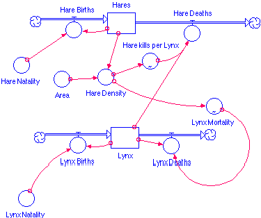
In order to model a predator vs. prey relationship we need to understand the relationships at work for each population and the interplay between the populations. Each population is dependent on the other and so whatever happens to one effects the other.

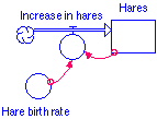
The simplest population model for a species would show no predators and exponential growth for the species. The population is dependent on a birth rate and the previous population. We can model that with a simple stock for the population, a flow for the increase in population into the stock, and a converter for the birth rate per species member.

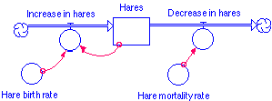
Eliminating members from the species requires a little more complexity. Usual cause for this is death of some sort. This can be modeled by a flow out of the population stock and a converter which contains the mortality rate of the species.

Most species must live within their present environment and so there are controlling factors for this. For instance, hares must have foliage and therefore acreage to live on and most likely the amount of acreage available is a limiting factor for the population. Lynx must have prey to eat and therefore prey in the habitat and most likely the amount of prey available is a limiting factor to the population growth.

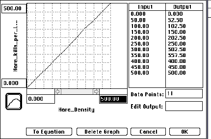
These limiting factors can usually be take care of by relating the birth or death rate to the limiting factor. Sometimes this is not a constant relationship but a varying one. Using a converter stock that has "become a graph" is one way to handle this variance.

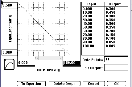
In this exercise we will attempt to first bring the populations into equilibrium by setting the initial values of our variables just so. Most populations, however, experience changing factors outside of those mentioned which throw their system out of equilibrium. Suppose, for instance, that a bounty is imposed on Lynx and many are killed in a short period of time. What changes can that impose on the balance between the populations?

We can simulate those sorts of changes through the use of "PULSE" functions. We would like to look at these as factors once we have a system in equilibrium.

Predator vs. Prey Equilibrium Problem

Assumptions:

Initial hare population of 50,000

Initial lynx population of 1,250

Initial hare birth rate of 1.25

Initial lynx birth rate of 1/5 of hare (.25)

Initial land area of 1,000 hectares (2,471 acres)

Stella pieces needed:

A stock for each population

A flow in to each stock and a flow out of each stock. One for increase due to birth and the other for decrease due to death.

Converter's for birth rates, acreage, mortality rates, lynx eating rates, and hare density.

All of the necessary connectors.

Formulas needed:

Simple products for the flows necessary for figuring the increase and decrease in populations (ex: hare birth rate * hares).

Quotient of hares and area for hare density.

"Become graph" functions for lynx mortality rate and lynx eating rate based on hare density.

Top level graphical interface:

A graph illustrating the populations of the two species for a period of at least 40 years.

A table showing the populations of the two species for each year.

Use your model to examine:

The initial values for the variables which will create a state of equilibrium for the populations.

Upsetting the Equilibrium

One way to program in such changes as bounties is to use the "PULSE" function. For this particular problem we want to add a converter called "Lynx Bounties" and connect it to the decrease in Lynx. In the formula for decrease in Lynx we will add to the end of the formula "+PULSE(Lynx_Bounties, 2,12)" . The second expression in the () represents when the first pulse takes place. The last represents the interval length before the next pulse. If entered as above, the bounties will be instituted every 12 time periods.

Check out the effects of varying the number of bounties and the time interval between.